E1 — A 2D portal frame

This is your first model with more than one member. A single-bay, single-storey moment-resisting portal frame — two columns and a beam — pushed sideways at the roof. It's the smallest model that still feels like a building: a lateral load goes in, a drift comes out, and the base reactions have to add back up to what you pushed with.

You already met the typed bridge on the cantilever. Everything here is the same spine — session → physical groups → apeSees(fem) → capture → read by name — but now you'll wire two element groups (columns and beam, with different sections), combine a gravity load with a lateral load, and pull two different answers back out: roof drift and base shear.

There's a twist worth flagging up front. When you check the drift against the hand calc you learned in school — the portal method — the FEM won't quite agree. That gap is not a bug. The FEM is the more correct of the two, and at the end we'll prove it by checking against a second, sharper hand calc.

The problem

        P = 60 kN                 W/2            W/2
        ───────►●═══════════════════════════════════●   ← roof (free to sway)
                ║                                     ║
                ║                                     ║   H = 5 m
                ║ columns                       beam  ║
                ║ 0.22 × 0.22                0.20×0.50║
              ██╨██                               ██╨██
              Fixed                               Fixed
              └────────────── B = 5 m ──────────────┘

  Material: steel, E = 200 GPa
  Lateral load P = 60 kN at the roof (+x)
  Gravity  W = 300 kN, split as two point loads on the roof joints (−y)

Two things we want out of this model:

Roof drift Δ. The classical back-of-the-envelope answer is the portal method: idealize the beam as rigid, so each fixed-base column behaves like a fixed–fixed shear column with lateral stiffness $k = 12EI_c/H^3$. Two columns in parallel give a storey stiffness $K = 2\cdot 12EI_c/H^3$, and

$$ \Delta_{\text{portal}} \;=\; \frac{P}{K} \;=\; \frac{P\,H^{3}}{24\,E\,I_c}. $$

With $I_c = \tfrac{0.22^4}{12} = 1.952\times10^{-4}\ \text{m}^4$, $P = 60\,000\ \text{N}$, $H = 5\ \text{m}$, $E = 200\times10^9\ \text{Pa}$, that's ≈ 8.00 mm.

Base shear. No formula needed — statics. The two column bases between them must react the entire applied lateral load, so the sum of the horizontal base reactions has to equal $P = 60\ \text{kN}$, exactly. That one is a sanity check the FEM has to pass to the last digit.

Units

Consistent SI throughout — metres, newtons, pascals. The drift comes out in metres because the geometry is in metres.

The whole model

The whole script, top to bottom. It's longer than the cantilever only because there are two members and two loads — the shape is identical. Read it once, then we'll walk it.

import numpy as np
from apeGmsh import apeGmsh, Results
from apeGmsh.opensees import apeSees, OpenSeesModel
from apeGmsh.results.capture.spec import DomainCaptureSpec

# --- Problem data (consistent SI: m, N, Pa) ---
H = 5.0                       # storey height   [m]
B = 5.0                       # bay width       [m]
E = 200e9                     # Young's modulus [Pa]  (steel)

bc, hc = 0.22, 0.22           # column section  [m]  (slim square)
Ac = bc * hc                  # column area     [m^2]
Ic = bc * hc**3 / 12.0        # column I        [m^4]

bb, hb = 0.20, 0.50           # beam section    [m]  (deeper, stiffer)
Ab = bb * hb                  # beam area       [m^2]
Ib = bb * hb**3 / 12.0        # beam I          [m^4]

P = 60_000.0                  # lateral roof load   [N]  (+x)
W = 300_000.0                 # total gravity load  [N]  (split on roof joints)

# --- 1. Geometry + physical groups ---
with apeGmsh(model_name="portal") as g:
    bl = g.model.geometry.add_point(0.0, 0.0, 0.0)   # base left
    br = g.model.geometry.add_point(B,   0.0, 0.0)   # base right
    tl = g.model.geometry.add_point(0.0, H,   0.0)   # roof left
    tr = g.model.geometry.add_point(B,   H,   0.0)   # roof right

    col_l = g.model.geometry.add_line(bl, tl)
    col_r = g.model.geometry.add_line(br, tr)
    beam  = g.model.geometry.add_line(tl, tr)
    g.model.sync()

    g.physical.add(1, [col_l, col_r], name="Columns")  # two columns -> one group
    g.physical.add(1, [beam],         name="Beam")     # the beam    -> its own group
    g.physical.add(0, [bl, br],       name="Base")     # fixed supports
    g.physical.add(0, [tl],           name="RoofL")    # load + drift readout
    g.physical.add(0, [tr],           name="RoofR")

    g.mesh.sizing.set_global_size(H / 6.0)
    g.mesh.generation.generate(1)
    fem = g.mesh.queries.get_fem_data(dim=1)

# --- 2. Build the OpenSees model through the typed bridge ---
ops = apeSees(fem)
ops.model(ndm=2, ndf=3)                    # 2-D frame: ux, uy, thetaz

transf = ops.geomTransf.Linear(vecxz=(0.0, 0.0, 1.0))
ops.element.elasticBeamColumn(pg="Columns", transf=transf, A=Ac, E=E, Iz=Ic)
ops.element.elasticBeamColumn(pg="Beam",    transf=transf, A=Ab, E=E, Iz=Ib)

ops.fix(pg="Base", dofs=(1, 1, 1))         # clamp both column bases

ts = ops.timeSeries.Linear()
with ops.pattern.Plain(series=ts) as pat:
    pat.load(pg="RoofL", forces=(P / 2.0, -W / 2.0, 0.0))   # half lateral + half gravity
    pat.load(pg="RoofR", forces=(P / 2.0, -W / 2.0, 0.0))

ops.constraints.Plain()
ops.numberer.Plain()
ops.system.BandGeneral()
ops.test.NormDispIncr(tol=1e-10, max_iter=10)
ops.algorithm.Linear()
ops.integrator.LoadControl(dlam=1.0)
ops.analysis.Static()

# --- 3. Solve, capturing roof displacement AND base reactions ---
spec = DomainCaptureSpec(opensees=ops)
spec.nodes(pg="RoofL", components=["displacement"])
spec.nodes(pg="RoofR", components=["displacement"])
spec.nodes(pg="Base",  components=["reaction_force"])
with ops.domain_capture(spec, path="run.h5") as cap:
    cap.begin_stage("lateral", kind="static")
    ops.analyze(steps=1)
    cap.step(t=1.0)
    cap.end_stage()

# --- 4. Read it back, by physical-group NAME ---
results = Results.from_native("run.h5", model=OpenSeesModel.from_h5("run.h5"))

dl = results.nodes.get(pg="RoofL", component="displacement_x")
dr = results.nodes.get(pg="RoofR", component="displacement_x")
drift_fem = 0.5 * (float(dl.values[-1, 0]) + float(dr.values[-1, 0]))

rx = results.nodes.get(pg="Base", component="reaction_force_x")
base_shear = float(rx.values[-1, :].sum())

# --- Drift check #1: the portal-method shortcut (rigid-beam) ---
drift_portal = P * H**3 / (24.0 * E * Ic)

print(f"drift_FEM    = {drift_fem*1e3:.4f} mm")
print(f"drift_portal = {drift_portal*1e3:.4f} mm")
print(f"gap          = {abs(drift_fem-drift_portal)/drift_fem*100:.2f} %")
print(f"base_shear   = {base_shear:.1f} N   (applied P = {P:.1f} N)")
print(f"shear error  = {abs(base_shear + P)/P*100:.6f} %")

Run it. You should see:

drift_FEM    = 8.3883 mm
drift_portal = 8.0041 mm
gap          = 4.58 %
base_shear   = -60000.0 N   (applied P = 60000.0 N)
shear error  = 0.000000 %

The base shear is exact: the horizontal base reactions sum to −60 000 N, equal and opposite to the 60 kN we pushed with. Equilibrium, to the last digit — the model is doing physics, not approximating it.

The drift is 8.39 mm, but the portal method said 8.00 mm — a 4.6 % gap. Hold that thought; we resolve it below.

Step 1 — Two physical groups, not one

    g.physical.add(1, [col_l, col_r], name="Columns")  # both columns
    g.physical.add(1, [beam],         name="Beam")
    g.physical.add(0, [bl, br],       name="Base")
    g.physical.add(0, [tl],           name="RoofL")
    g.physical.add(0, [tr],           name="RoofR")

The cantilever had one structural group ("Beam"). A frame has parts that behave differently, so we name them separately. "Columns" collects both column lines into a single group — they share a section, so they'll be one element declaration. "Beam" is its own group because it gets a different (deeper) section.

The two roof joints are named individually — "RoofL" and "RoofR" — so we can put a load on each and read each one's drift back. "Base" groups both fixed supports together.

This is the same discipline as before, just more of it: name every part you'll need to address later, and address it by that name from here on.

Step 2 — Two element groups, one transform

transf = ops.geomTransf.Linear(vecxz=(0.0, 0.0, 1.0))
ops.element.elasticBeamColumn(pg="Columns", transf=transf, A=Ac, E=E, Iz=Ic)
ops.element.elasticBeamColumn(pg="Beam",    transf=transf, A=Ab, E=E, Iz=Ib)

Here's the first genuinely new move. Two elasticBeamColumn calls — one per physical group, each with its own section properties. The "Columns" group becomes every column element with the column's A and Iz; the "Beam" group becomes the beam with the deeper section. One line per member type, the whole frame.

They share one geometric transform. For a planar frame all members live in the same plane, so a single Linear transform orients them all — you build it once and pass the same handle to both element declarations. (If your columns and beam needed different local-axis orientations — say in a 3-D frame — you'd build a transform per orientation and hand each group the one it needs.)

ops.fix(pg="Base", dofs=(1, 1, 1))

Both column bases, clamped in one call — dofs=(1, 1, 1) fixes $u_x, u_y, \theta_z$ at every node in "Base". Two fixed bases is what makes this a moment frame rather than a pinned-base sway frame.

Two loads in one pattern

ts = ops.timeSeries.Linear()
with ops.pattern.Plain(series=ts) as pat:
    pat.load(pg="RoofL", forces=(P / 2.0, -W / 2.0, 0.0))
    pat.load(pg="RoofR", forces=(P / 2.0, -W / 2.0, 0.0))

Both the lateral push and the gravity load live in the same Plain pattern, applied together at the two roof joints. Each joint takes half the lateral load ($+P/2$ in $x$) and half the gravity ($-W/2$ in $y$). The forces= tuple is (Fx, Fy, Mz) — a horizontal component, a vertical component, and zero applied moment.

Because both loads ramp together under one Linear series, the analysis applies a combined lateral-plus-gravity case in a single static step. Splitting them into separate patterns (dead, then lateral) is a later trick; for one combined check this is all you need.

The rest — constraints through analysis — is the standard linear-static analysis chain, identical to the cantilever.

Step 3 — Capture two different answers

spec = DomainCaptureSpec(opensees=ops)
spec.nodes(pg="RoofL", components=["displacement"])
spec.nodes(pg="RoofR", components=["displacement"])
spec.nodes(pg="Base",  components=["reaction_force"])

We want two distinct quantities, so we declare two kinds of capture. Displacement on the roof joints gives us drift. reaction_force on the base gives us the support reactions — the bridge calls ops.reactions() for you each step so the numbers are live. Three spec.nodes(...) calls, all targeted by name.

The solve block is unchanged from the cantilever: open a stage, run one static step in-process, snapshot, close.

Step 4 — Drift and base shear, by name

results = Results.from_native("run.h5", model=OpenSeesModel.from_h5("run.h5"))

dl = results.nodes.get(pg="RoofL", component="displacement_x")
dr = results.nodes.get(pg="RoofR", component="displacement_x")
drift_fem = 0.5 * (float(dl.values[-1, 0]) + float(dr.values[-1, 0]))

rx = results.nodes.get(pg="Base", component="reaction_force_x")
base_shear = float(rx.values[-1, :].sum())

Results.from_native(..., model=...) opens the run file (model in the same file — the Composed-file pattern, model= required). Then we read back by the same names we loaded: displacement_x on the two roof joints (we average them — in a symmetric sway they're equal anyway), and reaction_force_x on the base group.

The base group has two nodes, so rx.values[-1, :] is the last-step horizontal reaction at each base, and .sum() adds them — that's the total base shear the frame delivers to its foundations.

The 4.6 % gap is the lesson

So why is the FEM drift (8.39 mm) larger than the portal-method drift (8.00 mm)? Because the portal method lies to make the algebra easy. Its one big assumption — a rigid beam — pins the column tops against rotation. Real beams bend. When the beam flexes, the joints rotate, the columns lean further, and the frame is softer than the rigid-beam idealization predicts. A softer frame drifts more. The FEM models the beam's real stiffness, so it sees the extra flexibility the portal method threw away.

To prove the FEM is the trustworthy one — and not just different — drop the rigid-beam fiction and do the drift the rigorous way: slope-deflection, which carries the real bending stiffness of both the columns and the beam. By symmetry the frame has two unknowns — the joint rotation $\theta$ and the sway $\psi = \Delta/H$ — and a 2×2 system in $k_c = EI_c/H$, $k_b = EI_b/B$:

import numpy as np
kc, kb = E * Ic / H, E * Ib / B
A = np.array([[4*kc + 6*kb, -6*kc],
              [12*kc,        -24*kc]])
theta, psi = np.linalg.solve(A, np.array([0.0, P * H]))
drift_sd = abs(psi * H)
print(f"drift_FEM         = {drift_fem*1e3:.4f} mm")
print(f"drift_slope_defl  = {drift_sd*1e3:.4f} mm")
print(f"FEM vs slope-defl = {abs(drift_fem-drift_sd)/drift_sd*100:.3f} %")

drift_FEM         = 8.3883 mm
drift_slope_defl  = 8.3733 mm
FEM vs slope-defl = 0.179 %

0.18 %. Once the hand calc stops pretending the beam is rigid, it lands right on top of the FEM. The residual sliver that's left is the column axial shortening under gravity — which even slope-deflection ignores, but the FEM does not. So the ranking is:

Drift estimate	Value	What it captures
Portal method (rigid beam)	8.00 mm	columns only — beam idealized rigid
FEM (apeGmsh → OpenSees)	8.39 mm	columns + beam bending + axial
Slope-deflection (flexible beam)	8.37 mm	columns + beam bending

The portal method isn't wrong — it's a deliberately conservative-on-the- stiff-side preliminary tool, and 4.6 % is a fine first estimate to size a member. But this is exactly the kind of effect a real model is for: the FEM keeps the parts the hand formula drops. Treat the gap as a feature, and treat the slope-deflection agreement as your proof that the model is sound.

See it

results.plot.deformed(...) renders the warped shape headless (matplotlib, no GPU needed). Looking straight down the out-of-plane axis turns the planar frame into a clean elevation:

ax = results.plot.deformed(step=-1, scale=200)
ax.view_init(elev=90, azim=-90)     # look down +z -> 2-D elevation
ax.figure.savefig("portal-deformed.png", dpi=130, bbox_inches="tight")

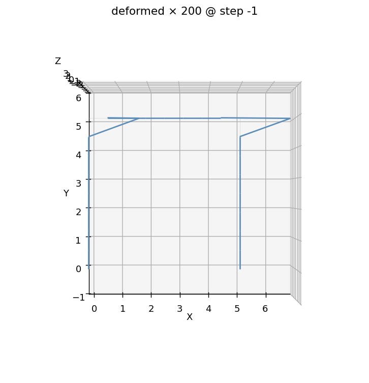
Both columns lean to the right, the roof translates as a unit, and the fixed bases stay put — the sway mode you'd sketch by hand, drawn straight from the result slab. (The displacements are magnified ×200; at true scale 8 mm over a 5 m frame is invisible.)

For an interactive 3-D view in a notebook, reach for results.show_web() — the kernel-safe web viewer. (Never call results.viewer() in a notebook; its blocking VTK+Qt loop crashes the kernel.)

What you just learned

This was the cantilever spine scaled up to a real structure:

• One physical group per behaviour. "Columns", "Beam", "Base", "RoofL", "RoofR" — name every part you'll address, then address it by name. Two columns share a group because they share a section; the beam gets its own.
• Multiple element groups, one transform. Two elasticBeamColumn calls, each pg= a different group with its own A/Iz, sharing one planar geomTransf.Linear.
• Combined loads in one pattern. Lateral and gravity at the roof joints, ramped together in a single Plain pattern.
• Capture more than one quantity. displacement for drift, reaction_force for base shear — declared by name, read by name.
• Base shear is statics. The base reactions summed to the applied load exactly — your free equilibrium check on any frame.
• The FEM beats the hand shortcut. The 4.6 % gap vs the portal method is the FEM capturing beam flexibility + axial that the rigid-beam idealization drops — confirmed by a 0.18 % match against slope-deflection.

Where next

• Multi-part assembly — build a column once as a Part, stamp it three times, and keep each instance addressable by its own label.
• Modal analysis — give a cantilever mass and pull its natural frequencies out through Results.

---

Next: Modal analysis of a cantilever.