E8 — Choosing a results strategy
Every example so far recorded its run the same way: in-process domain
capture, read back with Results.from_native. That's the right default,
and the tutorials pick it on purpose so you reach an answer without a
detour. But it isn't the only way OpenSees can hand you results, and sooner
or later you'll have a reason to choose differently — a colleague wants the
output in STKO, or you're driving a workflow built around classic
.out recorder files.
Here's the reassuring part, and the whole point of this page: the way you
read results never changes. results.nodes.get(pg="RoofL",
component="displacement_x") is the same call whether the numbers came from
a native capture, an MPCO file, or a stack of recorder .out files. You
pick a recording strategy; the reading code is identical. We'll prove it
by solving one model — the portal frame from E1 — two
different ways and watching the answers land on the same number to the last
digit.
Two axes, not one
"Results strategy" is really two independent choices:
from_native (capture) |
from_recorders (classic) |
from_mpco (STKO) |
|
|---|---|---|---|
Run in-process (ops.analyze) |
← the default | ✓ | ✓ |
Export a deck (ops.tcl / ops.py) |
✓ | ✓ | ✓ |
- How you run — solve in-process through openseespy (what every
example here does), or export a runnable deck (
ops.tcl("m.tcl")/ops.py("m.py")) and run it elsewhere. - How you record — domain capture (→
from_native), classic recorders writing.outfiles (→from_recorders), or an MPCO recorder for STKO (→from_mpco).
The read side is the same across the whole grid. This example holds the run axis fixed (in-process) and varies the record axis, so you can see the read code stay put while the recording changes underneath it.
There's a decision page for this
When you're choosing for real, the Choose a results strategy how-to walks the trade-offs (file size, STKO compatibility, restart-ability, coverage). This example is the proof that the choice doesn't touch your read code.
One read function, two recordings
The trick to seeing the symmetry is to write the read once and reuse it. Everything else — building the portal, configuring the analysis — is the E1 model verbatim, so we fold it into helpers and focus on the recording.
import os, tempfile
import numpy as np
from apeGmsh import apeGmsh, Results
from apeGmsh.opensees import apeSees, OpenSeesModel
from apeGmsh.results.capture.spec import DomainCaptureSpec
import openseespy.opensees as opspy

# --- Portal data (consistent SI: m, N, Pa) — same model as Example E1 ---
H, B, E = 5.0, 5.0, 200e9
bc, hc = 0.22, 0.22; Ac = bc*hc; Ic = bc*hc**3/12
bb, hb = 0.20, 0.50; Ab = bb*hb; Ib = bb*hb**3/12
P, W = 60e3, 300e3
work = tempfile.mkdtemp()

# --- The portal, built once (E1 geometry) ---
with apeGmsh(model_name="portal") as g:
    bl = g.model.geometry.add_point(0.0, 0.0, 0.0); br = g.model.geometry.add_point(B, 0.0, 0.0)
    tl = g.model.geometry.add_point(0.0, H, 0.0);   tr = g.model.geometry.add_point(B, H, 0.0)
    col_l = g.model.geometry.add_line(bl, tl); col_r = g.model.geometry.add_line(br, tr)
    beam  = g.model.geometry.add_line(tl, tr); g.model.sync()
    g.physical.add(1, [col_l, col_r], name="Columns"); g.physical.add(1, [beam], name="Beam")
    g.physical.add(0, [bl, br], name="Base"); g.physical.add(0, [tl], name="RoofL"); g.physical.add(0, [tr], name="RoofR")
    g.mesh.sizing.set_global_size(H/6.0); g.mesh.generation.generate(1)
    fem = g.mesh.queries.get_fem_data(dim=1)

def configure():
    """Build the portal on a fresh bridge through the analysis chain."""
    ops = apeSees(fem); ops.model(ndm=2, ndf=3)
    transf = ops.geomTransf.Linear(vecxz=(0.0, 0.0, 1.0))
    ops.element.elasticBeamColumn(pg="Columns", transf=transf, A=Ac, E=E, Iz=Ic)
    ops.element.elasticBeamColumn(pg="Beam",    transf=transf, A=Ab, E=E, Iz=Ib)
    ops.fix(pg="Base", dofs=(1, 1, 1))
    with ops.pattern.Plain(series=ops.timeSeries.Linear()) as pat:
        pat.load(pg="RoofL", forces=(P/2, -W/2, 0.0)); pat.load(pg="RoofR", forces=(P/2, -W/2, 0.0))
    ops.constraints.Plain(); ops.numberer.Plain(); ops.system.BandGeneral()
    ops.test.NormDispIncr(tol=1e-10, max_iter=10); ops.algorithm.Linear()
    ops.integrator.LoadControl(dlam=1.0); ops.analysis.Static()
    return ops

def read_drift(results):
    """The read side — IDENTICAL no matter how the run was recorded."""
    dl = results.nodes.get(pg="RoofL", component="displacement_x")
    dr = results.nodes.get(pg="RoofR", component="displacement_x")
    return 0.5 * (float(dl.values[-1, 0]) + float(dr.values[-1, 0]))

# --- Strategy 1: in-process domain capture -> Results.from_native ---
native = os.path.join(work, "run.h5")
ops = configure()
spec = DomainCaptureSpec(opensees=ops)
spec.nodes(pg="RoofL", components=["displacement"]); spec.nodes(pg="RoofR", components=["displacement"])
with ops.domain_capture(spec, path=native) as cap:
    cap.begin_stage("lateral", kind="static"); ops.analyze(steps=1); cap.step(t=1.0); cap.end_stage()
with Results.from_native(native, model=OpenSeesModel.from_h5(native, fem_root="/model")) as r:
    drift_native = read_drift(r)

opspy.wipe()   # clear the capture run before recording the MPCO run

# --- Strategy 2: MPCO recorder (STKO) -> Results.from_mpco ---
mpco = os.path.join(work, "run")              # OpenSees appends ".mpco"
model_h5 = os.path.join(work, "model.h5")
ops = configure()
ops.recorder.MPCO(file=mpco, nodal_responses=("displacement",))
ops.h5(model_h5)                              # sibling structural model for the read side
ops.run(wipe=False); opspy.analyze(1); opspy.wipe()   # wipe flushes the .mpco
with Results.from_mpco(mpco + ".mpco", fem=fem, model_h5=model_h5) as r:
    drift_mpco = read_drift(r)

print(f"from_native  drift = {drift_native*1e3:.4f} mm")
print(f"from_mpco    drift = {drift_mpco*1e3:.4f} mm")
print(f"agree to     {abs(drift_native-drift_mpco)*1e3:.2e} mm")
Run it. You should see:
Identical — to the last digit, zero difference. The portal swayed
8.3883 mm (exactly the E1 answer), and it didn't matter whether we read it
out of a native capture file or an MPCO file. read_drift never knew the
difference: it called results.nodes.get(pg="RoofL", ...) both times.
What actually changed
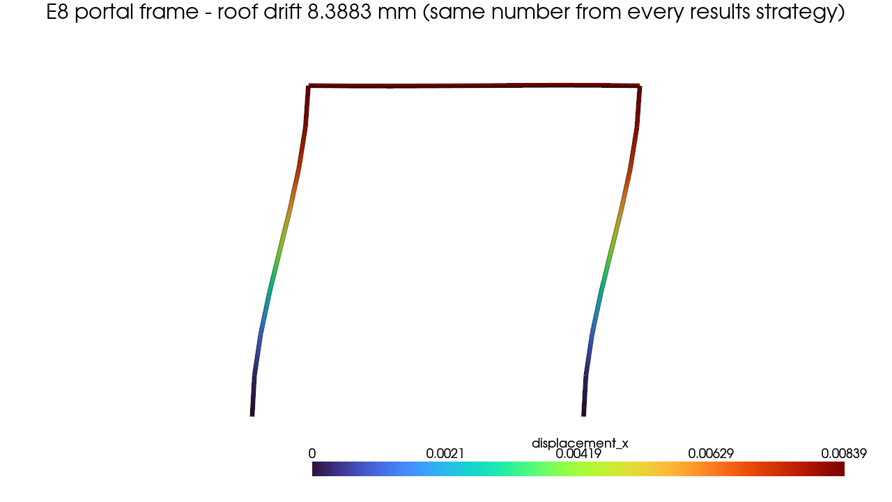
Look at what differs between the two strategies — it's only the recording:
Native capture declares a DomainCaptureSpec, opens an
ops.domain_capture(...) block around the solve, and reads with
Results.from_native(path, model=OpenSeesModel.from_h5(path, fem_root="/model")).
The model lives in the same file (the Composed-file pattern), and model=
is required so the broker can turn "RoofL" back into a node.
MPCO declares ops.recorder.MPCO(file=..., nodal_responses=("displacement",)),
writes a sibling structural model with ops.h5(...), runs the analysis, and
reads with Results.from_mpco(path, fem=fem, model_h5=model_h5).
Two things the MPCO path needs
model_h5=— an MPCO file carries only a partial model (no physical-group regions), sofrom_mpconeeds a siblingmodel.h5(written byops.h5(...)) to recover the structural side. Passfem=too so name-based queries (pg="RoofL") resolve.- Local disk — write the
.mpcoto local disk andwipe()in the same process before reading it. Pointing an MPCO recorder at a synced virtual drive (OneDrive / Dropbox / SeaDrive) can crash the kernel on close;HDF5_USE_FILE_LOCKING=FALSEdoes not fix it.
The read — read_drift — is byte-for-byte the same function applied to
both. That's the invariant worth internalising: your post-processing code
is decoupled from your recording choice.
The third strategy — classic recorders
The grid has a third column: classic OpenSees recorders that write plain
.out files, read back with Results.from_recorders. The read side is
still the same results.nodes.get(...):
# After running a deck whose recorders wrote .out files to `out_dir`:
om = OpenSeesModel.from_h5("model.h5")
with Results.from_recorders(spec, out_dir, fem=fem, model=om) as r:
    drift = read_drift(r)          # the SAME read function
This path shines when you're consuming the output of a Tcl/openseespy deck
someone else ran, or when you want the human-readable .out files on disk.
The mechanics of emitting the recorders and matching the files are covered in
the recorder reference and
the read displacement & reactions how-to.
What you just learned
- Recording and reading are independent. You choose how the run is
recorded (native capture / MPCO / classic recorders) separately from how
you read it back — and the read API (
results.nodes.get(pg=...,
  component=...)
) is identical across all three. - The default is
from_native(in-process domain capture) — fewest moving parts, broadest coverage, one Composed file. from_mpcogives you STKO-compatible output; it needs a siblingmodel.h5(ops.h5) +fem=to resolve names, and a local-disk path.from_recordersreads classic.outfiles — the path for consuming decks run elsewhere.- Proof, not promise: native and MPCO read the same portal drift, 8.3883 mm, to a difference of exactly zero.
Where next
- Portal frame — the E1 model this page re-solves, if you want the walkthrough behind the 8.39 mm.
- Choose a results strategy — the decision page: which column of the grid to pick, and why.
- Get results via MPCO — the MPCO recipe in isolation, with the STKO round-trip details.
Next: E9 — Compose modules.