Your first model in 10 minutes

You're going to build, solve, and inspect a real finite-element model end to end: a steel cantilever beam, fixed at one end, with a point load at the tip. By the end you'll have a deflection number you can trust — because you'll check it against a formula you already know by heart.

We pick a cantilever on purpose. It is the Hello, World of structural mechanics: one element type, one support, one load, and a closed-form answer that's been in every textbook for a century. If apeGmsh gets this right, you can believe what it tells you about the models that don't have closed-form answers.

The problem

        P = 10 kN  (downward)
                              |
                              v
  Fixed ████|=============================●  ← tip
        ████|                                   (free end)
        ████|<------------ L = 3 m ------------>|

  Section: 0.10 m × 0.20 m rectangle (strong axis bending)
  Material: steel, E = 200 GPa

A tip-loaded cantilever has a deflection you can write down without solving anything:

$$ \delta_{\text{tip}} \;=\; \frac{P\,L^{3}}{3\,E\,I} $$

With $P = 10{,}000\ \text{N}$, $L = 3\ \text{m}$, $E = 200\times10^{9}\ \text{Pa}$, and $I = \tfrac{b h^{3}}{12} = \tfrac{0.10 \cdot 0.20^{3}}{12} = 6.667\times10^{-5}\ \text{m}^4$:

$$ \delta_{\text{tip}} \;=\; \frac{10{,}000 \cdot 3^{3}}{3 \cdot 200\times10^{9} \cdot 6.667\times10^{-5}} \;=\; 6.75\times10^{-3}\ \text{m} \;=\; 6.75\ \text{mm} $$

Keep 6.75 mm in your back pocket. That's the number apeGmsh has to reproduce.

Units

apeGmsh is unit-agnostic — it stores the numbers you give it. We work in consistent SI throughout: metres, newtons, pascals. Pick a consistent system and stick to it; the deflection comes out in metres because the geometry is in metres.

Install

pip install "apeGmsh[all] @ git+https://github.com/nmorabowen/apeGmsh.git@main"

The [all] extra pulls in everything you need for this tutorial, including the web viewer. You also need OpenSees — apeGmsh drives it through openseespy, which [all] installs for you. (Not on PyPI yet — the line installs from the repo.) If you only want the modelling core, drop the [all], but this tutorial runs a real solve, so install [all].

The whole model

Here is the entire script. We'll walk through it block by block right after — but it's short enough to read top to bottom first, so do that. Under 40 lines of real work takes you from an empty session to a verified deflection.

from apeGmsh import apeGmsh, Results
from apeGmsh.opensees import apeSees, OpenSeesModel
from apeGmsh.results.capture.spec import DomainCaptureSpec

# --- Problem data (consistent SI: m, N, Pa) ---
L  = 3.0          # length        [m]
E  = 200e9        # Young's mod.   [Pa]  (steel)
b, h = 0.10, 0.20 # section sides  [m]
A  = b * h                  # area            [m^2]
Iz = b * h**3 / 12.0        # strong-axis I   [m^4]
P  = 10_000.0     # tip load       [N]  (downward, -y)

# --- 1. Geometry + physical groups, inside a session ---
with apeGmsh(model_name="cantilever") as g:
    p0   = g.model.geometry.add_point(0.0, 0.0, 0.0)
    p1   = g.model.geometry.add_point(L,   0.0, 0.0)
    beam = g.model.geometry.add_line(p0, p1)
    g.model.sync()

    g.physical.add(1, [beam], name="Beam")    # the line  -> elements
    g.physical.add(0, [p0],   name="Fixed")   # left end  -> support
    g.physical.add(0, [p1],   name="Tip")     # right end -> load + readout

    g.mesh.sizing.set_global_size(L / 10.0)   # ~10 line elements
    g.mesh.generation.generate(1)
    fem = g.mesh.queries.get_fem_data(dim=1)

# --- 2. Build the OpenSees model through the typed bridge ---
ops = apeSees(fem)
ops.model(ndm=2, ndf=3)                       # 2-D frame: ux, uy, thetaz

transf = ops.geomTransf.Linear(vecxz=(0.0, 0.0, 1.0))
ops.element.elasticBeamColumn(pg="Beam", transf=transf, A=A, E=E, Iz=Iz)

ops.fix(pg="Fixed", dofs=(1, 1, 1))           # clamp ux, uy, thetaz

ts = ops.timeSeries.Linear()
with ops.pattern.Plain(series=ts) as pat:
    pat.load(pg="Tip", forces=(0.0, -P, 0.0)) # downward point load

ops.constraints.Plain()
ops.numberer.Plain()
ops.system.BandGeneral()
ops.test.NormDispIncr(tol=1e-10, max_iter=10)
ops.algorithm.Linear()
ops.integrator.LoadControl(dlam=1.0)
ops.analysis.Static()

# --- 3. Solve, capturing the tip displacement ---
spec = DomainCaptureSpec(opensees=ops)
spec.nodes(pg="Tip", components=["displacement"])
with ops.domain_capture(spec, path="run.h5") as cap:
    cap.begin_stage("tip_load", kind="static")
    ops.analyze(steps=1)
    cap.step(t=1.0)
    cap.end_stage()

# --- 4. Read the result back by physical-group NAME ---
results = Results.from_native("run.h5", model=OpenSeesModel.from_h5("run.h5"))
slab = results.nodes.get(pg="Tip", component="displacement_y")

delta_fem = abs(float(slab.values[-1, 0]))
delta_exact = P * L**3 / (3.0 * E * Iz)
print(f"delta_FEM   = {delta_fem*1e3:.3f} mm")
print(f"delta_exact = {delta_exact*1e3:.3f} mm")
print(f"error       = {abs(delta_fem-delta_exact)/delta_exact*100:.4f} %")

Run it. You should see:

delta_FEM   = 6.750 mm
delta_exact = 6.750 mm
error       = 0.0000 %

That's our 6.75 mm, dead on. (The error is exactly zero, not just small: the elastic beam-column element carries the cubic bending shape exactly, so for a tip point load it is the closed-form solution — no discretization error to speak of.)

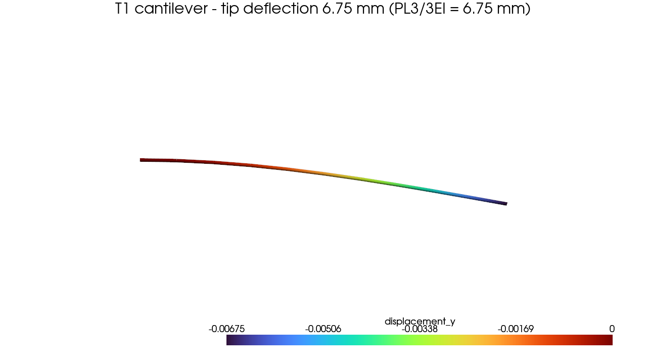
Now let's see why each block does what it does.

Step 1 — A session owns the geometry

with apeGmsh(model_name="cantilever") as g:
    p0   = g.model.geometry.add_point(0.0, 0.0, 0.0)
    p1   = g.model.geometry.add_point(L,   0.0, 0.0)
    beam = g.model.geometry.add_line(p0, p1)
    g.model.sync()

apeGmsh(...) opens a session — the live Gmsh kernel that owns your geometry and mesh. Everything you do to the model goes through composites hanging off g (here g.model.geometry). Using it as a context manager (with ... as g:) means the kernel is cleaned up for you when the block exits.

We place two points and a line between them — that's the whole geometry. The g.model.sync() flushes those operations into the kernel so the next steps can see them.

Physical groups: name the parts you care about

    g.physical.add(1, [beam], name="Beam")    # dim 1 = the curve
    g.physical.add(0, [p0],   name="Fixed")   # dim 0 = a point
    g.physical.add(0, [p1],   name="Tip")

This is the single most important habit in apeGmsh. A physical group is a named tag you attach to geometry — "Beam", "Fixed", "Tip". From here on you address everything by these names, never by raw entity numbers. Supports go on "Fixed", the load goes on "Tip", and when you read results back you ask for "Tip" again. The names survive meshing, solving, and post-processing — they are your handle on the model through every stage.

The first argument is the dimension: 1 for the line (which will become beam elements), 0 for the end points (which will become single nodes for the support and the load).

Mesh it

    g.mesh.sizing.set_global_size(L / 10.0)   # target element length
    g.mesh.generation.generate(1)             # 1 = mesh 1-D entities
    fem = g.mesh.queries.get_fem_data(dim=1)

We ask for a target element length of L/10, then generate(1) meshes the 1-D geometry into about ten line elements. (For a linear-elastic beam under a tip point load you'd get the exact answer with a single element — but ten keeps the picture honest and gives the viewer something to draw.)

The payoff line is get_fem_data(dim=1). This takes a snapshot of the meshed model — nodes, elements, and your physical groups, frozen into a FEMData object called fem. That snapshot is the bridge between the geometry world (inside the with) and the OpenSees world (outside it). Notice we grab it before the block closes, then carry it forward.

Step 2 — The typed OpenSees bridge

ops = apeSees(fem)
ops.model(ndm=2, ndf=3)

apeSees(fem) constructs the OpenSees bridge from your snapshot. This is how apeGmsh drives OpenSees: not by writing raw ops.element('...', ...) strings, but through typed primitives with real signatures your editor can autocomplete and your type checker can verify. You declare what you want; the bridge resolves your physical-group names against fem and emits a correct deck.

ops.model(ndm=2, ndf=3) must come first. We use a 2-D frame: 2 spatial dimensions, 3 degrees of freedom per node — horizontal, vertical, and an in-plane rotation ($u_x, u_y, \theta_z$). That rotation DOF is what makes this a beam and not a truss.

transf = ops.geomTransf.Linear(vecxz=(0.0, 0.0, 1.0))
ops.element.elasticBeamColumn(pg="Beam", transf=transf, A=A, E=E, Iz=Iz)

Every beam-column element needs a geometric transformation — the rule that maps the element's local axes to global ones. Linear is the small-deflection choice (exactly right for this elastic problem); the vecxz vector orients the local axes. The transform comes back as a handle — you pass the object itself, not a string name — and apeGmsh wires up the tags for you.

Then ops.element.elasticBeamColumn(pg="Beam", ...) writes every element in the "Beam" physical group as a linear-elastic beam-column with the area, modulus, and second moment we computed up top. One line, the whole member — because you targeted the group by name.

ops.fix(pg="Fixed", dofs=(1, 1, 1))

The clamp. dofs=(1, 1, 1) fixes all three DOFs (1 = fixed, 0 = free) at every node in "Fixed" — here that's the single left-end node. A fully-fixed end is exactly the cantilever boundary condition.

ts = ops.timeSeries.Linear()
with ops.pattern.Plain(series=ts) as pat:
    pat.load(pg="Tip", forces=(0.0, -P, 0.0))

Loads live inside a pattern. A Plain pattern scaled by a Linear time series ramps the load from zero to full over the analysis. pat.load(pg="Tip", ...) puts a force on every node in "Tip" — (0.0, -P, 0.0) is P newtons straight down (negative $y$), with no moment.

The remaining lines (constraints, numberer, system, test, algorithm, integrator, analysis) are the standard OpenSees analysis chain — the solver recipe. For a single linear step this is boilerplate; later tutorials explain when you'd reach for something other than Linear/Static.

What the bridge carries over for you

Two things you declare on the session reach the solver automatically: multi-point constraints and loads declared via g.loads. Here we declared the load the other way — directly on ops with pat.load — which is equally fine; just don't declare the same load both ways or you'll apply it twice. Masses and supports are always set on ops (ops.mass, ops.fix), so the runnable deck is explicit about them.

Step 3 — Solve and capture

spec = DomainCaptureSpec(opensees=ops)
spec.nodes(pg="Tip", components=["displacement"])
with ops.domain_capture(spec, path="run.h5") as cap:
    cap.begin_stage("tip_load", kind="static")
    ops.analyze(steps=1)
    cap.step(t=1.0)
    cap.end_stage()

We want the tip displacement, so we declare a capture spec: record the displacement of every node in "Tip". Again — by name.

ops.domain_capture(...) opens an in-process recorder writing to run.h5. Inside the with, we open a stage, run ops.analyze(steps=1) (one static load step — the solve happens here, in-process, through openseespy), snapshot the state with cap.step(t=1.0), and close the stage. When the block exits, run.h5 holds both the result and a copy of the model, in one file.

This is one path of several — on purpose

We did two things here that have alternatives, and this tutorial picks one of each so you reach a result without a detour:

• How you run — we solved in-process with ops.analyze. You can instead export a runnable deck with ops.tcl("model.tcl") or ops.py("model.py") and run it elsewhere (great for sharing or version-controlling the OpenSees model).
• How you record — we used domain capture (→ Results.from_native). You can also use classic recorders (→ Results.from_recorders) or an MPCO recorder for STKO (→ Results.from_mpco).

The read-side API is identical whichever you choose. When you're ready to pick, see the results & export recipes — you don't need them to finish here.

Step 4 — Read it back, by name

results = Results.from_native("run.h5", model=OpenSeesModel.from_h5("run.h5"))
slab = results.nodes.get(pg="Tip", component="displacement_y")
delta_fem = abs(float(slab.values[-1, 0]))

Results.from_native(...) opens the run file. The model= argument is required — Results needs a model broker to translate physical-group names back into nodes and elements. Here the model lives in the same file (the Composed-file pattern), so we point OpenSeesModel.from_h5 at the same path.

Then the moment of truth: results.nodes.get(pg="Tip", component="displacement_y"). You ask for the vertical displacement of the "Tip" group — the same name you used to apply the load — and get back a typed slab of values. slab.values[-1, 0] is the last step, first (and only) tip node. We take the magnitude, print it next to PL³/3EI, and watch them match.

This is the payoff of naming everything: you never once touched a raw node number. The model, the load, and the readout all speak the same language — your physical-group names.

See it

results.show_web()

results.show_web() launches the notebook-safe web viewer — an interactive 3-D view of the deformed shape, right in your Jupyter output cell. Use this one in notebooks.

Don't pass blocking=True in a notebook

results.viewer() defaults to blocking=None (auto): scripts get the in-process Qt window; a Jupyter / VS Code kernel spawns a subprocess (or show_web() for in-memory Results). An explicit blocking=True still runs a native VTK + Qt event loop that crashes the kernel. In a notebook, results.show_web() is the interactive choice.

What you just learned

In one short script you ran the entire apeGmsh spine:

• Session → geometry → physical groups. Open a session, draw the geometry, and name the parts you care about with g.physical.add(...). Those names are your handle on the model forever after.
• get_fem_data is the snapshot. It freezes the meshed model into a FEMData object that carries your names across the boundary into OpenSees.
• The typed bridge. apeSees(fem) drives OpenSees through typed primitives — ops.geomTransf.Linear, ops.element.elasticBeamColumn, ops.fix(pg=...), ops.pattern.Plain — never raw command strings.
• Capture → Results → read by name. ops.domain_capture records the solve; Results.from_native(..., model=...) reads it back; results.nodes.get(pg=...) pulls displacements out by physical-group name.
• show_web() for the picture, and it's the kernel-safe choice in notebooks.

And the model checks out — 6.75 mm, exactly PL³/3EI.

Where next

• A plate in tension — the same typed bridge on a 2-D solid: nDMaterial, a tension field, and stresses you read back by physical group.
• The SS beam, the apeGmsh way — meet the loads/masses/sections composites: declare a distributed load once and let apeGmsh resolve the tributary work for you.
• Save, reload, view — persist a model to disk and reopen it, and the full notebook-safe results loop.
• Core mental model — the six ideas behind everything you just did, on one page.

---

Next: A plate in tension.