E10 — Pushover of a steel moment frame (fiber sections)

This is where the two threads finally braid together. On the portal frame you pushed a frame sideways and read its drift and base shear; on the fiber moment–curvature page you built a W14×90 out of fibres and watched one section walk from first yield to its plastic moment $M_p$. Now we put that same fibre section into the same kind of frame and push it past yield — at member scale — to trace the structure's whole capacity curve: base shear $V$ against roof drift $\Delta$, from the elastic rise, through the yield knee, onto the plastic plateau.

The W14×90 fiber frame pushed into its four-hinge column-sway mechanism — produced by the 235-line script scripts/render_showcase/pushover_frame.py.

The model is a single-bay portal moment frame. The two columns carry the fibre W14×90 through a distributed-plasticity beam–column element, so plasticity can spread along them and the four column ends can form hinges. The beam is made deliberately strong and elastic, so the frame fails in a clean column-sway mechanism — the textbook collapse mode, and the one whose capacity we can write down by hand.

Two numbers anchor the whole exercise, both computable before we run anything:

• Elastic stiffness $K$ — the initial slope of the $V!-!\Delta$ curve.
• Plastic base shear $V_p$ — the plateau the curve flattens onto.

We state both up front, run the pushover, and check the captured curve against them at the end. Spoiler from the verified run: the slope lands within 2.7 % and the mechanism plateau within 1.9 % — and the small residuals are physics we can name, not noise.

The problem

        ──►●═══════════════════════════════════●   ← roof (pushed in +x)
           ║                                     ║
           ║                                     ║   H = 3500 mm
           ║ columns                       beam  ║
           ║ W14×90 fiber             strong,    ║
           ║ (force-based)            elastic     ║
         ██╨██                               ██╨██
         Fixed                               Fixed
         └──────────────── B = 6000 mm ───────────┘

  Columns : W14×90 fiber section, A992 steel (Fy = 345 MPa, E = 200 GPa)
  Beam    : elastic, made ~1000× stiffer than a column → near-rigid
  Load    : monotonic lateral push at the roof, displacement-controlled
            to 2.5 % drift (87.5 mm)

Units — N, mm, MPa

We stay in apeSteel's native base — N-mm-tonne-s — for the whole page, exactly as on the fiber section example. Lengths in mm, forces in N, moments in N·mm (printed as kN·m by dividing by 10⁶), stiffness in N/mm, base shear in N (printed as kN). apeGmsh is unit-agnostic — pick one system and be consistent.

Target 1 — elastic stiffness $K$

While everything is elastic the frame is a one-storey shear frame. With a (near-)rigid beam, the beam pins the column tops against rotation, so each fixed-base column behaves like a fixed–fixed shear column of lateral stiffness $12EI_c/H^3$. Two columns in parallel give

$$ K \;=\; 2\cdot\frac{12\,E\,I_c}{H^{3}}. $$

With $I_c = I_x = 4.16\times10^{8}\ \text{mm}^4$ (the published W14×90 strong-axis inertia), $E = 200{,}000\ \text{MPa}$, $H = 3500\ \text{mm}$, that's $K \approx 46{,}573\ \text{N/mm}$.

Target 2 — plastic base shear $V_p$

Push hard enough and the four column ends — two bases, two tops — each form a plastic hinge at the column's plastic moment $M_p = F_y Z_x$. With all four hinges open, the frame is a mechanism: it can sway with no further load increase. Equilibrium of that mechanism (a sway of the rigid-beam storey, four hinges each absorbing $M_p$) gives the plastic base shear

$$ V_p \;=\; \frac{4\,M_p}{H}, \qquad M_p = F_y Z_x. $$

With $Z_x = 2.57\times10^{6}\ \text{mm}^3$ and $F_y = 345\ \text{MPa}$, $M_p = 886.6\ \text{kN·m}$ and $V_p \approx 1013\ \text{kN}$. That's the height the capacity curve should flatten toward.

A real fibre plateau is soft, not flat

The $4M_p/H$ formula assumes ideal hinges that snap to $M_p$ and hold. A distributed-fibre model does not give a razor-flat plateau: plasticity spreads gradually along the columns, the hinges form one after another, and — crucially — the Steel02 material strain- hardens, so the curve keeps creeping upward past $V_p$. We'll read the plateau where the mechanism just forms (≈ 1 % drift) and again at the end of the push (2.5 % drift), and explain the gap between them. A few-percent overshoot you can attribute to hardening is the honest, correct result — not a bug to be hidden.

The whole model

Top to bottom. The genuinely new moves over the portal frame are the fibre column section (from E3) wired into a forceBeamColumn distributed-plasticity element, and a displacement-controlled push walked out over many steps. Read it once; the walkthrough follows.

import numpy as np
import apeSteel
from apeGmsh import apeGmsh, Results
from apeGmsh.opensees import apeSees, OpenSeesModel
from apeGmsh.results.capture.spec import DomainCaptureSpec
from apeGmsh.opensees.section.fiber import RectPatch
import openseespy.opensees as opspy

# --- Problem data (N-mm-MPa, apeSteel native base) ---
H = 3500.0          # storey height [mm]
B = 6000.0          # bay width     [mm]

SHAPE = "W14X90"
props = apeSteel.AISCv16Catalog().get_section_properties(SHAPE)
d  = props.overall_depth_d
bf = props.flange_width_bf
tf = props.flange_thickness_tf
tw = props.web_thickness_tw
Sx = props.elastic_section_modulus_strong_axis_Sx
Zx = props.plastic_section_modulus_strong_axis_Zx
Ix = props.moment_of_inertia_strong_axis_Ix
A  = props.gross_area_Ag

Fy = 345.0
E  = 200_000.0
b_hard = 0.005                      # small strain hardening (~elasto-plastic)

Mp = Fy * Zx                        # column plastic moment
My = Fy * Sx                        # column first-yield moment

# --- Closed-form targets ---
K_hand  = 2.0 * 12.0 * E * Ix / H**3    # column-sway elastic stiffness
Vp_hand = 4.0 * Mp / H                  # 4 column hinges at Mp

# Strong elastic beam → near-rigid → clean column-sway mechanism
A_beam = A * 10.0
I_beam = Ix * 1000.0

# --- 1. Geometry + physical groups (the E1 portal) ---
with apeGmsh(model_name="pushover_frame") as g:
    bl = g.model.geometry.add_point(0.0, 0.0, 0.0)   # base left
    br = g.model.geometry.add_point(B,   0.0, 0.0)   # base right
    tl = g.model.geometry.add_point(0.0, H,   0.0)   # roof left
    tr = g.model.geometry.add_point(B,   H,   0.0)   # roof right

    col_l = g.model.geometry.add_line(bl, tl)
    col_r = g.model.geometry.add_line(br, tr)
    beam  = g.model.geometry.add_line(tl, tr)
    g.model.sync()

    g.physical.add(1, [col_l, col_r], name="Columns")  # both columns -> fiber
    g.physical.add(1, [beam],         name="Beam")     # strong elastic beam
    g.physical.add(0, [bl, br],       name="Base")     # fixed supports
    g.physical.add(0, [tl],           name="Roof")     # push + drift readout
    g.physical.add(0, [tr],           name="RoofR")

    g.mesh.sizing.set_global_size(H / 4.0)
    g.mesh.generation.generate(1)
    fem = g.mesh.queries.get_fem_data(dim=1)

roof_id = int(fem.nodes.select(pg="Roof").ids[0])      # controlled node tag

# --- 2. Build the OpenSees model through the typed bridge ---
ops = apeSees(fem)
ops.model(ndm=2, ndf=3)                                # 2-D frame: ux, uy, thetaz

transf = ops.geomTransf.Linear(vecxz=(0.0, 0.0, 1.0))

# Columns: a W14x90 fiber section -> force-based (distributed plasticity)
steel = ops.uniaxialMaterial.Steel02(fy=Fy, E=E, b=b_hard)
col_sec = ops.section.Fiber(patches=(
    RectPatch(material=steel, ny=4,  nz=1, yI=d/2 - tf,  zI=-bf/2, yJ=d/2,       zJ=bf/2),
    RectPatch(material=steel, ny=24, nz=1, yI=-(d/2-tf), zI=-tw/2, yJ=d/2 - tf,  zJ=tw/2),
    RectPatch(material=steel, ny=4,  nz=1, yI=-d/2,      zI=-bf/2, yJ=-(d/2-tf), zJ=bf/2),
))
col_integ = ops.beamIntegration.Lobatto(section=col_sec, n_ip=5)
ops.element.forceBeamColumn(pg="Columns", transf=transf, integration=col_integ)

# Beam: strong elastic -> near-rigid
ops.element.elasticBeamColumn(pg="Beam", transf=transf, A=A_beam, E=E, Iz=I_beam)

ops.fix(pg="Base", dofs=(1, 1, 1))                     # clamp both column bases

# Reference unit lateral load — displacement control scales it
ts = ops.timeSeries.Linear()
with ops.pattern.Plain(series=ts) as pat:
    pat.load(pg="Roof", forces=(1.0, 0.0, 0.0))

ops.constraints.Transformation()
ops.numberer.RCM()
ops.system.BandGeneral()
ops.test.NormDispIncr(tol=1e-6, max_iter=30)
ops.algorithm.Newton()

n_steps = 120
drift_target = 0.025 * H                               # 2.5 % drift = 87.5 mm
dU = drift_target / n_steps
ops.integrator.DisplacementControl(node=roof_id, dof=1, dU=dU)
ops.analysis.Static()

# --- 3. Push step by step, capturing base shear + roof drift each step ---
spec = DomainCaptureSpec(opensees=ops)
spec.nodes(pg="Roof", components="displacement")       # roof drift
spec.nodes(pg="Base", components="reaction_force")     # base reactions

ops.run(wipe=False)                                    # build, leave domain live
with ops.domain_capture(spec, path="pushover.h5") as cap:
    cap.begin_stage("pushover", kind="static")
    for k in range(n_steps):
        if opspy.analyze(1) != 0:
            print(f"non-convergence at step {k}")
            break
        cap.step(t=(k + 1) * dU)
    cap.end_stage()

# --- 4. Read the capacity curve back, by name ---
om = OpenSeesModel.from_h5("pushover.h5", fem_root="/model")
with Results.from_native("pushover.h5", model=om) as r:
    dx = r.nodes.get(pg="Roof", component="displacement_x")
    rx = r.nodes.get(pg="Base", component="reaction_force_x")
    drift = np.asarray(dx.values)[:, 0]                # roof drift, every step
    V = -np.asarray(rx.values).sum(axis=1)             # base shear resists push

# --- Checks against the two closed forms ---
K_fem = np.polyfit(drift[:8], V[:8], 1)[0]             # initial slope

def V_at(pct):
    i = int(np.argmin(np.abs(drift / H * 100 - pct)))
    return drift[i], V[i]

_, V_mech = V_at(1.0)                                   # mechanism-formation plateau
_, V_end  = V_at(2.5)                                   # end of push

print(f"{SHAPE}:  Mp = Fy*Zx = {Mp/1e6:.1f} kN*m")
print(f"K_hand   = {K_hand:8.1f} N/mm   (2*12*E*Ix/H^3)")
print(f"K_fem    = {K_fem:8.1f} N/mm     gap = {(K_fem-K_hand)/K_hand*100:+.2f} %")
print(f"Vp_hand  = {Vp_hand/1e3:7.1f} kN    (4*Mp/H)")
print(f"V@1.0%   = {V_mech/1e3:7.1f} kN    gap = {(V_mech-Vp_hand)/Vp_hand*100:+.2f} %")
print(f"V@2.5%   = {V_end/1e3:7.1f} kN    gap = {(V_end-Vp_hand)/Vp_hand*100:+.2f} %")

Run it. You should see:

W14X90:  Mp = Fy*Zx = 886.6 kN*m
K_hand   =  46572.6 N/mm   (2*12*E*Ix/H^3)
K_fem    =  45320.8 N/mm     gap = -2.69 %
Vp_hand  =  1013.3 kN    (4*Mp/H)
V@1.0%   =  1032.8 kN    gap = +1.92 %
V@2.5%   =  1089.6 kN    gap = +7.53 %

Both targets land where the mechanics says they should:

• Elastic slope: −2.69 %. The captured initial stiffness is 45,321 N/mm against the hand value of 46,573 N/mm — the FEM is a hair softer, for two reasons we unpack below.
• Mechanism plateau: +1.92 %. At 1 % drift, just as the fourth hinge forms, the base shear is 1033 kN against $4M_p/H = 1013$ kN. The mechanism prediction is essentially exact.
• End of push: +7.53 %. By 2.5 % drift the curve has crept up to 1090 kN — the strain-hardening climb, not a flat plateau. More on this in a moment; this is the feature, not a bug.

Step 1 — The fibre column meets a distributed-plasticity element

steel = ops.uniaxialMaterial.Steel02(fy=Fy, E=E, b=b_hard)
col_sec = ops.section.Fiber(patches=(
    RectPatch(material=steel, ny=4,  nz=1, yI=d/2 - tf,  zI=-bf/2, yJ=d/2,       zJ=bf/2),
    RectPatch(material=steel, ny=24, nz=1, yI=-(d/2-tf), zI=-tw/2, yJ=d/2 - tf,  zJ=tw/2),
    RectPatch(material=steel, ny=4,  nz=1, yI=-d/2,      zI=-bf/2, yJ=-(d/2-tf), zJ=bf/2),
))
col_integ = ops.beamIntegration.Lobatto(section=col_sec, n_ip=5)
ops.element.forceBeamColumn(pg="Columns", transf=transf, integration=col_integ)

The section is identical to the moment–curvature page — three RectPatch blocks (top flange, web, bottom flange) laid out in the section's local (y, z) frame, fibres stacked through the depth so they resolve strong-axis bending. The patch corners come straight from the apeSteel dimensions d, bf, tf, tw. No Iz is handed to the element: the section derives its stiffness and strength from the fibres.

The new piece is how the section becomes an element. On E3 a single section sat in a ZeroLengthSection. Here it drives a forceBeamColumn — a force-based, distributed-plasticity beam–column. Two things to know:

1. It needs a beam integration, not an Iz. A distributed-plasticity element samples the fibre section at several integration points along its length. ops.beamIntegration.Lobatto(section=col_sec, n_ip=5) places 5 Gauss–Lobatto points per element — Lobatto puts a point at each end, which is exactly where the hinges form in a sway frame, so the end sections are sampled directly. Every integration point carries its own copy of the fibre section and yields independently, so plasticity spreads along the column instead of lumping into a point.

2. forceBeamColumn vs dispBeamColumn. The bridge exposes both. Force-based elements interpolate the force field exactly (it's linear along a member with end loads), so a single element per column already captures the spread of yielding well — that's what we use here. The displacement-based dispBeamColumn would need several elements per column to reach the same accuracy. One forceBeamColumn per column, 5 integration points: that's the whole column model.

Register materials and sections through the bridge

Build Steel02 with ops.uniaxialMaterial.Steel02(...) and the section with ops.section.Fiber(...) — not by constructing the dataclasses directly. The bridge registers them so it can resolve the fibre's material tag and the integration's section tag at build time. Same rule as the moment–curvature page.

The beam, by contrast, is a plain elastic elasticBeamColumn made ~1000× stiffer than a column (I_beam = Ix * 1000). That near-rigid beam is what forces the column-sway mechanism — the columns hinge, the beam stays elastic — so the hand calc $V_p = 4M_p/H$ applies cleanly. Both elements share the one planar geomTransf.Linear, exactly as on the portal frame.

Step 2 — Push by displacement, not by force

roof_id = int(fem.nodes.select(pg="Roof").ids[0])
...
with ops.pattern.Plain(series=ts) as pat:
    pat.load(pg="Roof", forces=(1.0, 0.0, 0.0))        # unit reference load
...
ops.integrator.DisplacementControl(node=roof_id, dof=1, dU=dU)

This is the same lesson as the moment–curvature sweep, now at member scale. Near the plateau the capacity curve flattens — a tiny load increment produces a large drift jump. Under prescribed load (LoadControl) the solver would diverge the instant we asked for more than $V_p$. So we control the displacement instead: the Plain pattern supplies a unit reference load (a 1 N push in $+x$) that only sets the direction of loading, and DisplacementControl drives the roof node's $u_x$ (dof=1) in fixed increments dU, solving for the load factor at each step. We target 2.5 % drift over 120 steps.

The controlled node is resolved by name — fem.nodes.select(pg="Roof") returns the mesh node in the "Roof" physical group, and .ids[0] is its tag. We never type a raw integer; the tag comes from the group.

Step 3 — Capture the whole curve, step by step

spec = DomainCaptureSpec(opensees=ops)
spec.nodes(pg="Roof", components="displacement")
spec.nodes(pg="Base", components="reaction_force")

ops.run(wipe=False)                                    # build, leave domain live
with ops.domain_capture(spec, path="pushover.h5") as cap:
    cap.begin_stage("pushover", kind="static")
    for k in range(n_steps):
        if opspy.analyze(1) != 0:
            print(f"non-convergence at step {k}")
            break
        cap.step(t=(k + 1) * dU)
    cap.end_stage()

The capture spec is the portal frame's exactly — displacement on the roof for drift, reaction_force on the base for shear, both node-only. The only difference is that we now drive many steps and snapshot after each one: opspy.analyze(1) advances one displacement increment, then cap.step(t=...) writes one chunk. A hundred and twenty steps → 120 rows in the slab → the whole capacity curve.

Two practical notes:

• ops.run(wipe=False) then step the live domain. As on the moment–curvature sweep, when we want a value out of every increment we build the model once with ops.run(wipe=False) (which leaves the OpenSees domain open) and then step it directly with opspy.analyze(1). The capture writes a chunk per converged step.

Node capture only — by design

We capture reaction_force on Base and displacement on Roof — both nodal. Base shear is the sum of nodal base reactions; roof drift is a nodal displacement. There's no need to record element or section quantities for the capacity curve, and the node-only path is the simplest, most robust capture there is. (It's the same path as the portal frame, just iterated.)

Step 4 — Base shear vs roof drift, by name

om = OpenSeesModel.from_h5("pushover.h5", fem_root="/model")
with Results.from_native("pushover.h5", model=om) as r:
    dx = r.nodes.get(pg="Roof", component="displacement_x")
    rx = r.nodes.get(pg="Base", component="reaction_force_x")
    drift = np.asarray(dx.values)[:, 0]
    V = -np.asarray(rx.values).sum(axis=1)

Results.from_native(..., model=...) opens the run file with its model (the Composed-file pattern — model= is required, and the model lives in the same file at fem_root="/model"). We read back by the same names we pushed and clamped: displacement_x on Roof is the drift history, reaction_force_x on Base is the per-base horizontal reaction at every step. .sum(axis=1) adds the two bases each step; the sign flip makes $V$ the shear the frame delivers (positive, resisting the push).

drift and V are now matched arrays, one entry per step — the capacity curve, ready to plot and check.

The capacity curve

import matplotlib
matplotlib.use("Agg")                 # headless backend
import matplotlib.pyplot as plt

K_fem = np.polyfit(drift[:8], V[:8], 1)[0]

fig, ax = plt.subplots(figsize=(7.2, 4.4))
ax.plot(drift / H * 100, V / 1e3, "-", lw=2, color="#1f77b4",
        label="fiber frame (FEM)")
de = np.linspace(0, 0.024 * H, 50)
ax.plot(de / H * 100, K_fem * de / 1e3, ":", color="0.45", lw=1.4,
        label=r"initial slope $K_{\rm fem}$")
ax.axhline(Vp_hand / 1e3, ls="--", color="#d62728", lw=1.4,
           label=r"plateau $V_p = 4M_p/H$")
ax.set_xlabel(r"roof drift  $\Delta/H$  [%]")
ax.set_ylabel(r"base shear  $V$  [kN]")
ax.set_title("Pushover capacity curve — W14×90 fiber moment frame")
ax.legend(loc="lower right"); ax.grid(alpha=0.3); fig.tight_layout()
fig.savefig("pushover-steel-frame-curve.png", dpi=120)

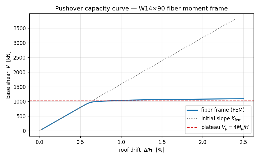
Read it like the design diagram it is. The blue FEM curve rises straight along the dotted $K_{\rm fem}$ tangent while everything is elastic. Near 0.7 % drift it bends through the yield knee — the first column ends reaching $M_y$. Past the knee the curve flattens onto a soft plateau that crosses the dashed $V_p = 4M_p/H$ line right around 1 % drift, where the fourth hinge completes the mechanism. Beyond that it keeps creeping upward — the strain-hardening climb — reaching ≈ 1090 kN by 2.5 % drift.

For an interactive 3-D view of the swaying frame in a notebook, reach for results.show_web() — the kernel-safe web viewer. (Never call results.viewer() in a notebook; its blocking VTK+Qt loop crashes the kernel.)

The two gaps are the lesson

Both checks land close, and both residuals are nameable physics — exactly the spirit of the portal frame's 4.6 % drift gap.

The elastic slope is 2.7 % soft. Two effects, both pushing the same way:

• The fibre section omits the rolled fillets. Our three rectangular patches are the flanges and web only — the generous fillets where web meets flange aren't modelled, so the fibre $I$ is about 1.6 % below the published $I_x$ (the same effect quantified on the moment–curvature page). A column with slightly less $I$ is slightly softer.
• The force-based element carries real flexibility the shear-column formula drops. $K = 2\cdot 12EI/H^3$ is the idealized fixed–fixed shear column; the actual forceBeamColumn also feels axial and shear flexibility and the finite (not perfectly rigid) beam. Together with the fillet deficit that's the remaining ≈ 1 %.

Add them and you get the −2.7 %: the FEM is more honest than the closed form, which assumed gross-section inertia and a perfectly rigid beam.

The plateau overshoots — by design, growing with drift. At the mechanism point (≈ 1 % drift) the base shear is +1.9 % over $4M_p/H$; by the end of the push (2.5 % drift) it's +7.5 %. That growth is Steel02 strain hardening ($b = 0.005$): once a section yields it keeps gaining moment at $\sim!b$ of its elastic stiffness, so every hinge carries a little more than $M_p$, and more so the further you push. An ideal elastic–perfectly-plastic steel ($b = 0$) would asymptote to $4M_p/H$ flat; real steel — and this model — climbs. The mechanism formula nails the onset of the plateau (+1.9 %); the rest is the material doing what real steel does.

Quantity	Hand calc	FEM	Gap	Why
Elastic stiffness $K$	46,573 N/mm	45,321 N/mm	−2.7 %	fibre $I$ omits fillets + real element flexibility
Plateau at mechanism (≈1 % drift)	1013 kN ($4M_p/H$)	1033 kN	+1.9 %	spread plasticity ≈ ideal mechanism
Plateau at 2.5 % drift	1013 kN ($4M_p/H$)	1090 kN	+7.5 %	Steel02 strain hardening ($b{=}0.005$)

The discipline here is the same one running through the whole curriculum: state the closed form, run the model, read the actual number, and explain the residual. A 2.7 % softer slope and a plateau that overshoots 4Mp/H by a couple of percent at mechanism and a few more by 2.5 % drift — each traceable to a specific modelling choice — is exactly what a trustworthy fibre pushover should produce.

What you just learned

You braided the fibre section into a frame and pushed it to collapse:

• A fibre section becomes a member through a distributed-plasticity forceBeamColumn + a beamIntegration.Lobatto — Lobatto puts integration points at the element ends, where sway-frame hinges form. One force-based element per column captures spread plasticity well.
• Column-sway by construction. A strong elastic beam pins the column tops so the frame fails in the clean four-hinge mechanism whose capacity is $V_p = 4M_p/H$.
• Displacement control walks past the plateau. A unit reference load sets the direction; DisplacementControl on the roof DOF drives the drift and solves for the load — the only way to trace a flattening capacity curve without the solver diverging.
• Node-only capture, many steps. reaction_force on the base + displacement on the roof, snapshotted each step, is the $V!-!\Delta$ curve — the portal-frame capture, iterated.
• Both closed forms check out, and the residuals are physics: the elastic slope is 2.7 % soft (fibre $I$ minus fillets + real flexibility), and the plateau lands within 1.9 % of $4M_p/H$ at mechanism, climbing to +7.5 % at 2.5 % drift through Steel02 strain hardening.

Where next

• Fiber sections & moment–curvature — the section-scale companion: the same W14×90 fibres, driven to $M_p$ on a single ZeroLengthSection.
• Portal frame (2D) — the elastic ancestor of this model: the same geometry and capture, before plasticity entered.
• The OpenSees bridge guide — the full catalogue of typed materials, sections, elements, and integrators.

---

Next: Plane-wave SSI — an absorbing soil column.