Save it, reload it, view it

You already know how to build a model, solve it, and read a number back — that's T1 and T3. This tutorial is the day-two workflow nobody shows you: you built the model on Monday, the OpenSees run takes an hour, and on Tuesday you want to reopen the thing, re-solve from exactly where you left off, and look at the deformed shape in your notebook without the kernel dying.

So we don't introduce a single new piece of mechanics. We take the simply-supported beam from T3 — the same span, section, support, and load — and learn three things instead:

1. how a session saves itself to a native .h5 when the with block closes,
2. how FEMData.from_h5 reloads that file with an integrity check, and
3. why Results needs a model=, and which viewer is safe to call in a notebook.

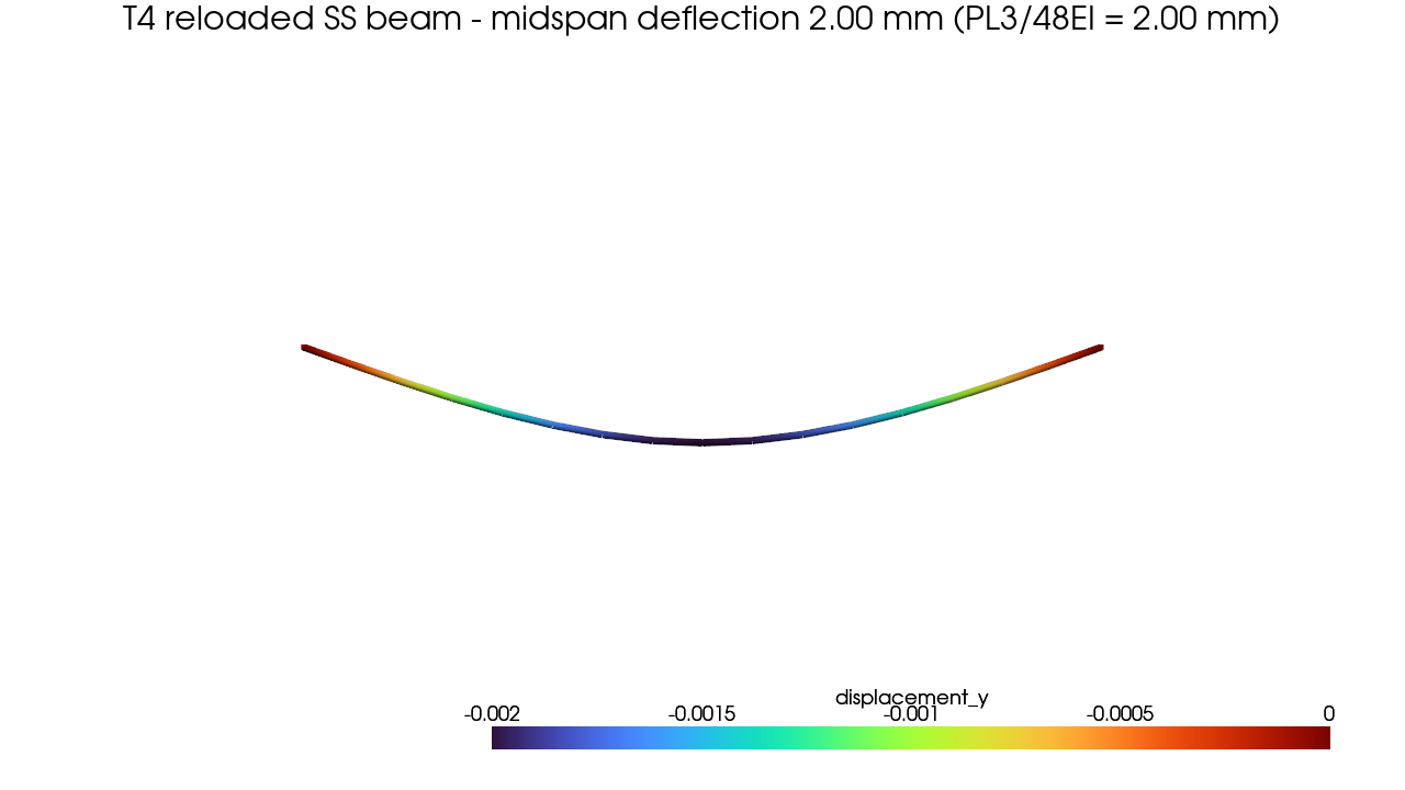
The check at the end is the whole point of persistence: the reloaded model has to reproduce the T3 midspan deflection identically — not close, identically — and the file's content hash has to prove nothing got corrupted on the round-trip.

The problem (a quick recap from T3)

                 P = 20 kN  (downward)
                          |
                          v
       ●===================●===================●
      △                  (mid)                 ○
   pin (ux, uy)                          roller (uy)
       |<------ L/2 ------>|<------ L/2 ------>|
       |<--------------- L = 4 m ------------->|

  Section: 0.10 m × 0.20 m rectangle (strong-axis bending)
  Material: steel, E = 200 GPa

A central point load on a simply-supported beam has a midspan deflection straight out of the textbook:

$$ \delta_{\text{mid}} \;=\; \frac{P\,L^{3}}{48\,E\,I} $$

With $P = 20{,}000\ \text{N}$, $L = 4\ \text{m}$, $E = 200\times10^{9}\ \text{Pa}$, and $I = \tfrac{b h^{3}}{12} = \tfrac{0.10 \cdot 0.20^{3}}{12} = 6.667\times10^{-5}\ \text{m}^4$:

$$ \delta_{\text{mid}} \;=\; \frac{20{,}000 \cdot 4^{3}}{48 \cdot 200\times10^{9} \cdot 6.667\times10^{-5}} \;=\; 2.00\times10^{-3}\ \text{m} \;=\; 2.00\ \text{mm} $$

Keep 2.00 mm in your back pocket. This is the number the model has to give us after it has been to disk and back.

Units

As always, consistent SI — metres, newtons, pascals. The deflection comes out in metres.

The whole script

Here is the entire thing. Read it top to bottom — the new lines are the persistence ones (save_to=, FEMData.from_h5); everything else you've seen in T1 and T3. We walk through it block by block right after.

from apeGmsh import apeGmsh, FEMData, Results
from apeGmsh.opensees import apeSees, OpenSeesModel
from apeGmsh.results.capture.spec import DomainCaptureSpec

# --- Problem data (consistent SI: m, N, Pa) ---
L  = 4.0          # span           [m]
E  = 200e9        # Young's mod.    [Pa]  (steel)
b, h = 0.10, 0.20 # section sides   [m]
A  = b * h                  # area            [m^2]
Iz = b * h**3 / 12.0        # strong-axis I   [m^4]
P  = 20_000.0     # midspan load    [N]  (downward, -y)

# --- 1. Build the model AND autosave it to a native .h5 on exit ---
with apeGmsh(model_name="ssbeam", save_to="ssbeam.h5", overwrite=True) as g:
    p0 = g.model.geometry.add_point(0.0,   0.0, 0.0)
    pm = g.model.geometry.add_point(L/2.0, 0.0, 0.0)   # split at midspan
    p1 = g.model.geometry.add_point(L,     0.0, 0.0)
    sl = g.model.geometry.add_line(p0, pm)
    sr = g.model.geometry.add_line(pm, p1)
    g.model.sync()

    g.physical.add(1, [sl, sr], name="Beam")     # the two curves -> elements
    g.physical.add(0, [p0], name="Pin")          # left support
    g.physical.add(0, [p1], name="Roller")       # right support
    g.physical.add(0, [pm], name="Mid")          # load + readout node

    g.mesh.sizing.set_global_size(L / 16.0)
    g.mesh.generation.generate(1)
    fem = g.mesh.queries.get_fem_data()          # full snapshot (every dim)
    snap_built = fem.snapshot_id                 # remember its content hash
    # ssbeam.h5 is written HERE, as the `with` block exits.

print(f"built    snapshot_id = {snap_built}")

# --- 2. Reload the model from disk — integrity-checked ---
fem2 = FEMData.from_h5("ssbeam.h5")
print(f"reloaded snapshot_id = {fem2.snapshot_id}")
print(f"hash match           = {fem2.snapshot_id == snap_built}")

# --- 3. Build + solve OpenSees from the RELOADED snapshot ---
ops = apeSees(fem2)
ops.model(ndm=2, ndf=3)

transf = ops.geomTransf.Linear(vecxz=(0.0, 0.0, 1.0))
ops.element.elasticBeamColumn(pg="Beam", transf=transf, A=A, E=E, Iz=Iz)

ops.fix(pg="Pin",    dofs=(1, 1, 0))    # pin:    ux, uy held
ops.fix(pg="Roller", dofs=(0, 1, 0))    # roller: uy held only

ts = ops.timeSeries.Linear()
with ops.pattern.Plain(series=ts) as pat:
    pat.load(pg="Mid", forces=(0.0, -P, 0.0))   # central point load

ops.constraints.Plain()
ops.numberer.Plain()
ops.system.BandGeneral()
ops.test.NormDispIncr(tol=1e-10, max_iter=10)
ops.algorithm.Linear()
ops.integrator.LoadControl(dlam=1.0)
ops.analysis.Static()

# --- 4. Capture, read back by name, and CHECK against T3 ---
spec = DomainCaptureSpec(opensees=ops)
spec.nodes(pg="Mid", components=["displacement"])
with ops.domain_capture(spec, path="ssbeam_run.h5") as cap:
    cap.begin_stage("midspan_load", kind="static")
    ops.analyze(steps=1)
    cap.step(t=1.0)
    cap.end_stage()

results = Results.from_native(
    "ssbeam_run.h5", model=OpenSeesModel.from_h5("ssbeam_run.h5"),
)
slab = results.nodes.get(pg="Mid", component="displacement_y")

delta_reload = abs(float(slab.values[-1, 0]))
delta_exact  = P * L**3 / (48.0 * E * Iz)
print(f"delta_reload = {delta_reload*1e3:.4f} mm")
print(f"delta_exact  = {delta_exact*1e3:.4f} mm")
print(f"error        = {abs(delta_reload-delta_exact)/delta_exact*100:.4f} %")

Run it. You should see:

built    snapshot_id = ac230fece5973edfadc9ab919a23daf5
reloaded snapshot_id = ac230fece5973edfadc9ab919a23daf5
hash match           = True
delta_reload = 2.0000 mm
delta_exact  = 2.0000 mm
error        = 0.0000 %

Two things just got proven. The two snapshot_id lines are identical — the model you saved is byte-for-content the model you reloaded. And the deflection is 2.00 mm, exactly PL³/48EI, computed from a model that spent a moment on disk. (As in T1, the elastic beam-column carries the cubic bending shape exactly, so there's no discretization error — the only thing being tested here is that persistence didn't change a single number.)

Now the why.

Step 1 — A session can save itself

with apeGmsh(model_name="ssbeam", save_to="ssbeam.h5", overwrite=True) as g:
    ...
    fem = g.mesh.queries.get_fem_data()
    snap_built = fem.snapshot_id
    # ssbeam.h5 is written HERE, as the `with` block exits.

The geometry is the only thing genuinely new versus T1: we drop a point at midspan (pm) and build the beam from two curves, sl and sr, so there's a real mesh node sitting exactly at the load point. Both curves go into the one "Beam" physical group; the midspan point becomes "Mid". Standard T3 setup.

The persistence is in the constructor: save_to="ssbeam.h5". This arms an autosave — when the with block exits (or you call g.end()), apeGmsh writes the meshed model to a native .h5 file. overwrite=True says it's fine to clobber an existing ssbeam.h5; with overwrite=False, an existing target raises FileExistsError so you can't trample a file by accident.

Autosave fires on exit, and only warns if it fails

Two things to internalise. First, save_to= does not write eagerly — nothing hits disk until end()/__exit__. If the process dies inside the with block, you get nothing. Second, the autosave on exit catches and warns on a write failure (so Gmsh can still finalize cleanly) rather than raising — a failed autosave can slip by as a warning. When persistence actually matters, call g.save() explicitly inside the block:

g.save()              # checkpoint now, to the save_to= target
g.save("ckpt.h5")     # ...or to an explicit path

g.save() with neither an explicit path nor a save_to= set raises RuntimeError — it won't guess where to put your model.

What gets saved — and the snapshot you check against

Notice we grab fem with a bare get_fem_data() — no dim= filter. That's deliberate. The autosave writes the whole meshed model: the 16 line elements of "Beam" and the three point "elements" that back the "Pin", "Roller", and "Mid" physical groups. To compare apples to apples after reload, the snapshot we remember (snap_built) has to be that same full model — so we take the full snapshot here. (Filter to dim=1 for the solve if you like; the beam elements are the same either way. We just keep one canonical snapshot so the hashes line up cleanly.)

fem.snapshot_id is a 32-character content hash over everything in the snapshot — nodes, elements, physical groups, labels, constraints, loads, masses. Two snapshots with identical content produce the identical hash. That's the property the next step leans on.

save_to/g.save() write the neutral model only

The native .h5 from g.save() holds the apeGmsh neutral zone — geometry, mesh, names — and no OpenSees deck. That's exactly what you want for "save the model, decide how to analyse it later." If you also want the OpenSees side (transforms, recorders) in the file, that's a different call — apeSees(fem).h5(path) writes a two-zone file (neutral + /opensees/). We don't need it here, but it's the same family of API.

Step 2 — Reload, with an integrity check baked in

fem2 = FEMData.from_h5("ssbeam.h5")
print(f"reloaded snapshot_id = {fem2.snapshot_id}")
print(f"hash match           = {fem2.snapshot_id == snap_built}")

FEMData.from_h5(path) rebuilds a full FEMData snapshot from the file — nodes, elements, physical groups, labels, the lot. No live Gmsh session is involved; the snapshot is self-sufficient, which is the entire reason it round-trips.

The important part is invisible: from_h5 re-verifies the file's /meta/snapshot_id. On read it recomputes the content hash of the rebuilt model and compares it against the hash stored when the file was written. If a single coordinate had been tampered with, it would raise MalformedH5Error('snapshot_id mismatch') rather than hand you a quietly corrupted model. That's why our two printed hashes match: the file is intact, and the reloaded model is the model we built.

from_h5 is fail-loud by design

A missing /meta group raises MalformedH5Error; a file written by a too-new schema raises SchemaVersionError. apeGmsh would rather refuse to open a file than silently feed you a wrong model. You don't have to do anything to opt in — the check runs on every from_h5.

There's a second flavour of reload worth knowing about (we don't use it here, but you'll meet it the day you assemble models):

g2 = apeGmsh.from_h5("ssbeam.h5")   # a *chain-phase* session, no gmsh

Mind the difference: FEMData.from_h5 gives you a snapshot; apeGmsh.from_h5 gives you a session — but a chain-phase one with no live Gmsh kernel behind it. You can g2.compose(...) other saved models onto it and g2.save(...) the result, but g2.model.* and g2.mesh.generation.* will fail (there's no kernel to draw into). For "reload one model and analyse it," FEMData.from_h5 is the tool — that's what we use.

Step 3 — Solve from the reloaded snapshot

ops = apeSees(fem2)            # <- the RELOADED snapshot, not the original
ops.model(ndm=2, ndf=3)
transf = ops.geomTransf.Linear(vecxz=(0.0, 0.0, 1.0))
ops.element.elasticBeamColumn(pg="Beam", transf=transf, A=A, E=E, Iz=Iz)
ops.fix(pg="Pin",    dofs=(1, 1, 0))
ops.fix(pg="Roller", dofs=(0, 1, 0))

This is pure T3 — and that's the lesson. apeSees(fem2) builds the typed bridge from fem2, the snapshot that just came off disk, and every physical-group name still works: "Beam", "Pin", "Roller", "Mid". The names survived the round-trip, so the bridge resolves them exactly as it would have on the live session.

The supports are the only physics difference from the T1 cantilever, and they're textbook simply-supported: the "Pin" holds ux and uy (dofs=(1, 1, 0), rotation free), the "Roller" holds only uy (dofs=(0, 1, 0)). The load, pattern, and analysis chain are the same shape you saw in T1.

Step 4 — Capture, read by name, and the viewer that won't crash

spec = DomainCaptureSpec(opensees=ops)
spec.nodes(pg="Mid", components=["displacement"])
with ops.domain_capture(spec, path="ssbeam_run.h5") as cap:
    cap.begin_stage("midspan_load", kind="static")
    ops.analyze(steps=1)
    cap.step(t=1.0)
    cap.end_stage()

results = Results.from_native(
    "ssbeam_run.h5", model=OpenSeesModel.from_h5("ssbeam_run.h5"),
)
slab = results.nodes.get(pg="Mid", component="displacement_y")

Same one capture-and-read path as T1: declare a DomainCaptureSpec for the "Mid" displacement, run one static step in-process, and the run file ssbeam_run.h5 ends up holding both the result and a copy of the model.

Results.from_native(...) opens it — and the model= argument is required. This trips people up, so it's worth saying plainly: Results stores numbers against raw node and element ids. To let you ask for "Mid" instead of a tag, it needs a model broker to translate names into ids. That broker is OpenSeesModel. Here the model rides inside the same run file (the Composed-file pattern), so we point OpenSeesModel.from_h5 at the same path. Omit model= and you get a TypeError — it's not optional, by design.

Then the payoff: results.nodes.get(pg="Mid", component="displacement_y") hands back the vertical displacement at the "Mid" group — the same name we loaded — and slab.values[-1, 0] is the last step at the one midspan node. Magnitude, print, compare to PL³/48EI. 2.00 mm, dead on, from a model that has been to disk and back.

See it — the notebook-safe way

results.show_web()

results.show_web() launches the notebook-safe web viewer — an interactive 3-D view of the deformed beam, rendered right in your Jupyter output cell. In a notebook, this is the one to reach for.

Don't pass blocking=True in a notebook

results.viewer() defaults to blocking=None (auto): scripts get the in-process Qt window; a Jupyter / VS Code kernel spawns a subprocess (or show_web() for in-memory Results) — the same hazard T1 used to warn about under the old default. An explicit blocking=True still crashes the kernel. In a notebook, use results.show_web(). (At a real terminal, the desktop viewer is fine; results.viewer(blocking=False) still forces the subprocess.)

What you just learned

You did a full build → save → reload → solve → view loop, and the reloaded model reproduced the answer exactly:

• save_to= arms an autosave that writes a native .h5 when the session's with block exits. It writes the neutral model (geometry, mesh, names) — no OpenSees needed. For a guaranteed checkpoint mid-session, call g.save() explicitly; the autosave only warns on failure.
• FEMData.from_h5 reloads with an integrity check. It re-verifies the stored snapshot_id against the rebuilt model and raises MalformedH5Error on any corruption — so a clean reload is a proven clean reload. Don't confuse it with apeGmsh.from_h5, which returns a kernel-less chain-phase session for composing saved models.
• Names survive the round-trip. "Beam", "Pin", "Mid" all resolve on the reloaded snapshot exactly as on the live one — which is why apeSees(fem2) is identical to building from the original.
• Results needs model=. The model broker is what turns stored ids back into your physical-group names; it's a required argument, not a convenience.
• show_web() for the picture in a notebook — and never the blocking results.viewer(), which crashes the kernel.

And the round-trip checks out: the same snapshot_id, and 2.00 mm — exactly PL³/48EI — after the model has been saved and reopened.

Where next

• T3 · A simply-supported beam, the apeGmsh way — if you skipped it, this is where the loads/masses/sections composites are taught; T4 reused its beam without re-deriving the mechanics.
• Results & export recipes — the alternatives we deliberately didn't fork into here: exporting a runnable Tcl/Py deck, classic recorders, and STKO .mpco files.
• Composing saved models — where apeGmsh.from_h5 earns its keep: reload several saved .h5 models and g.compose(...) them into one assembly.
• Core mental model — the ideas behind the snapshot, the broker, and the name-everything habit, on one page.

---

The tutorials end here; the example ladder starts with the portal frame. Next: A 2D portal frame.